Tutorial 2: Modal Analysis¶

In this tutorial we want do a modal analysis. It is applied on the example from the first tutorial. If you are not familiar with how to set up a MechanicalSystem instance, new materials and meshes, it is recommended to read Tutorial 1: Static Problem first.

Problem¶

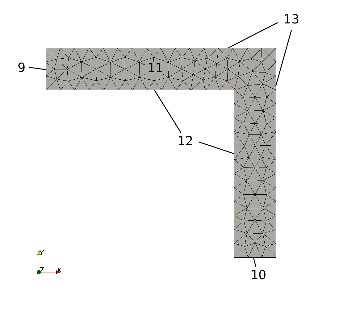
Fig. 2 Mesh of pressure corner.

Fig. 2 shows a meshed 2D corner. It is meshed by the open-source software Gmsh. You can find the Mesh-File in AMfe’s examples folder. Every edge and every surface is associated with a physical-group-number. The surface of the corner has the physical-group-number 11. The small edges belong to physical group 9 and 10, and the outer and inner edges belong to physical group 13 and 12, respectively.

It is the same geometry as in Tutorial 1: Static Problem. Now we are not interested in a static solution for a given Neumann-boundary-condition. We want to know the first ten eigenfrequencies of the pressure corner.

Solving the problem with AMfe¶

Setting up new simulation, mesh and material¶

As we have the same geometry, mesh and materials as in Tutorial 1: Static Problem, we enter the same commands:

import amfe
my_system = amfe.MechanicalSystem()
input_file = amfe.amfe_dir('meshes/gmsh/pressure_corner.msh')
output_file = amfe.amfe_dir('results/pressure_corner/pressure_corner_modes')
my_material = amfe.KirchhoffMaterial(E=210E9, nu=0.3, rho=7.86E3, plane_stress=True, thickness=0.1)
my_system.load_mesh_from_gmsh(input_file, 11, my_material)
my_system.apply_dirichlet_boundaries(9, 'x')
my_system.apply_dirichlet_boundaries(10, 'y')

Todo

Check if parameter 2 in Mesh is correctly described (see Tutorial 1)

Note

In this example we do not apply any Neumann boundary conditions because they would not be considered in modal analysis. Modal analysis with prestress has not been implemented yet.

Solve¶

The function vibration_modes(MechanicalSystem, save=True) solves the eigenproblem to the linearized system:

omega, V = amfe.vibration_modes(my_system, n=10, save=True)

The first parameter is the MechanicalSystem instance of the problem. The second parameter gives the number of vibration modes one is interested in and the last parameter is a flag that activates saving the modes for paraview export.

For viewing the results one can either use the returned variables (here omega and phi) or one can export the results to paraview. via:

my_system.export_paraview(output_file)

Results¶

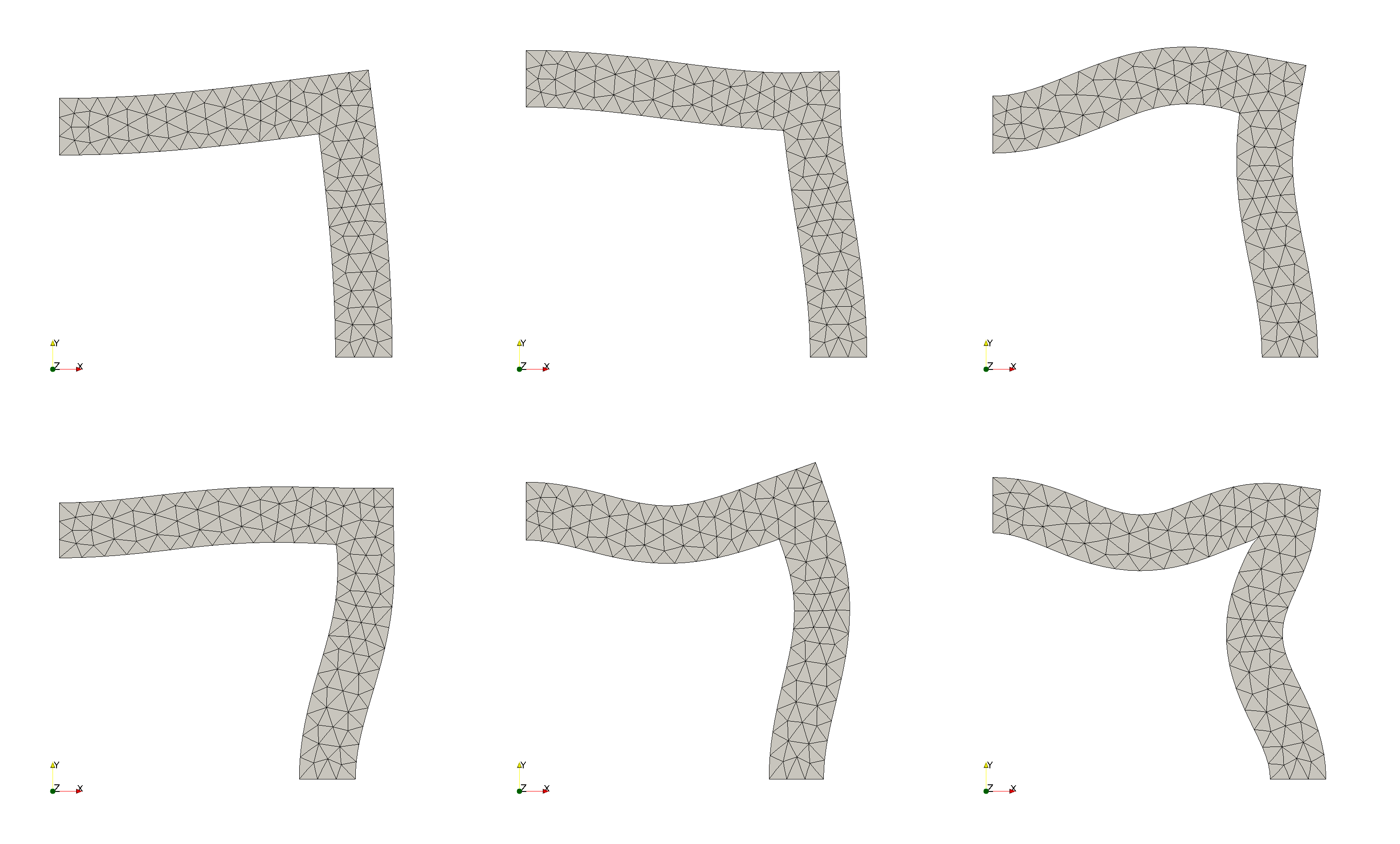
Fig. 3 First six modes of linearized pressure corner. Top: Modes 1-3, Bottom: Modes 4-6

Fig. 3 shows the first six modes of the linearized pressure corner.

The eigenfequencies in Hertz:

import numpy as np
f = omega/(2*np.pi)
f
array([  125.88198294,   296.66446201,   921.61100677,   994.45027039,
      1316.94610541,  1634.31575078,  2441.74646491,  2990.53919312,
      3530.41461115,  3688.88210744])